6 MIN READ - The Cautious Optimism Correspondent for Economic Affairs and Other Egghead Stuff ponders the likeliness that the Federal Reserve’s aggressive coronavirus easing will spark runway inflation.
 |
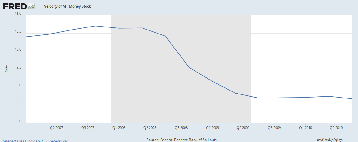
| Monetary Velocity: 2008-2015 |
Note: This analysis applies fundamental principles concerning the effects of money, output, and velocity on prices and inflation. For a primer on the basics of inflation go to:
http://www.cautiouseconomics.com/2020/04/monetary-policy-11.html
Since mid-March the Federal Reserve has flooded the financial system with new liquidity more quickly than during the depths of the 2008 financial crisis. Newly created reserves are being loaned out by commercial banks and multiplied into higher demand deposit balances.
So won’t all this new money spark massive inflation? Is our money doomed to go the way of the Venezuelan bolivar and become toilet paper?
In the Economics Correspondent’s opinion, the short answer is “very unlikely” although he won’t rule out a mild increase particularly in the near term—but not Weimar Republic Germany or Robert Mugabe’s Zimbabwe.
Some of the new money will spill over into asset markets, driving up the value of stocks and other securities which—while introducing a different set of risks longer term—have little effect on consumer prices and aren’t measured in official inflation statistics.
However the greatest counterbalance to the Fed’s monetary inflation will be falling monetary velocity which the Correspondent believes the Fed already considers a fait accompli.
X. OFFSETTING FALLING VELOCITY
There is no question the Federal Reserve is aggressively creating new bank reserves through extremely large asset purchases. In the March 11 to April 22 period total commercial bank reserves held at the Fed have risen from $1.72 trillion to $3.1 trillion, an increase of 80% in 42 days and a new record eclipsing the $2.8 trillion set in July of 2014 (see table 1, "Reserve balances with Federal Reserve Banks").
https://www.federalreserve.gov/releases/h41/current/h41.htm
The monetary base is also in record territory (see graph).
https://fred.stlouisfed.org/series/BOGMBASEW
Incidentally the rate of increase of both has slowed considerably from the operations’ frantic opening days.
The broader M1 aggregate, which reflects currency and commercial bank demand deposits (themselves the product of banks lending out reserves) has risen from $4.07 trillion to a record $4.52 trillion or up a more modest 11%.
https://fred.stlouisfed.org/series/M1
The even broader M2 aggregate has risen by $1.2 trillion during the same period from $15.66 trillion to $16.87 trillion, up even slower: 7.7%.
https://fred.stlouisfed.org/series/M2
But as we’ve already reviewed in the previous chapter on the Equation of Exchange (mv = py), final prices are influenced not only by changes in the money supply, but also by fluctuations in economic output (real GDP) and monetary velocity.
As we enter a major recession due to government social-distancing shutdowns and consumer fears of coronavirus infection, real output is sure to fall. Given that prices move in inverse proportion to output, a decline in real GDP will trigger an increase in prices.
So if, for example, the next quarterly GDP report reflects an epic annualized decline of 40%, then all things being equal the actual drop for the quarter itself (when not extracted on an annual basis) of 11.2% will propel a price inflation of 12.6% for the quarter alone.
Unnerving indeed. So why the downplayed inflation concerns?
Because—and this is a key concept—a fall in monetary velocity produces the opposite effect, a decline in prices. We have a recent example.
During the financial crisis single-year period 2Q2008 to 2Q2009 monetary velocity fell by 17% (see graph).
https://fred.stlouisfed.org/graph/fredgraph.png?g=qLgs
A 17% decline in velocity, all things being equal, will deflate prices by 17%. And applying the Equation of Exchange (mv = py) a 17% decline in velocity paired with an 11% increase in M1 and an 12.6% decline in output actually translates to a final inflation rate of 3.7%.
Now of course this is just a mathematical hypothetical using apples and oranges—a full year’s deflation, a quarterly GDP contraction, and a 42 days change in money supply. We don’t know yet what the M1 and GDP numbers will be by the end of the year, but the Economics Correspondent believes the Fed anticipates an even larger drop in velocity than 17% for 2020 and that the decline will easily outpace GDP’s in ensuing years as GDP resumes growth more rapidly than velocity.
The reasons aren’t hard to fathom.
Starting with a baseline of the 2008 financial crisis and its single-year 17% decline we can start making adjustments accounting for the more extreme economic conditions of the coronavirus crisis.
1) With nearly all of America under shutdown, consumers can’t spend on discretionaries and even some consumer staples, even if they have the means to do so.
2) Tens of millions of Americans will lose their jobs in the short-term. The lack of income will drive velocity down further.
3) Even when the lockdown restrictions are loosened, those Americans who still have jobs will forgo spending to bolster their savings as they worry about job security.
4) Even when the lockdown restrictions are loosened, Americans will be less willing to spend on most goods and services than before. Spending on travel, hospitality, restaurants, sporting events, many brick-and-mortal retail stores, personal fitness clubs, movie theaters—the list goes on and on—will fall to depressed levels until a cure or vaccine is widely available.
It doesn’t stop with consumers.
5) Firms have borrowed heavily and built liquid cash cushions to ride out the slump. However those reserves will be spent at a slower rate than before. With demand down across the board firms will be paying fewer workers, cutting back on operations, and abstaining from large capital investment projects.
The federal government is attempting to prop up spending and velocity with its $2+ trillion “life support” package, but borrowing and handing out trillions of dollars every month is unsustainable.
XI. RECOVERY
What about when the economy recovers?
Recent history shows in recessions GDP always bottoms out and recovers before velocity does.
In the 2008-09 recession, GDP bottomed out at about -5% in 2Q2009 before resuming growth at a very modest pace. However velocity’s fall remained persistent. By the end of 2015 velocity had declined by a whopping 44% and as of this article’s writing has still never reached a trough (see graphs).
https://fred.stlouisfed.org/graph/fredgraph.png?g=qNMS
https://fred.stlouisfed.org/graph/fredgraph.png?g=qNMP
Once again we can apply the Equation of Exchange.
Had the money supply remained constant from 2008 to 2015, prices would have fallen by 50% resulting in widespread bankruptcies as borrowers found it twice as difficult to earn the dollars needed to pay back fixed nominal debts.
In the 2000-01 recession, GDP bottomed out at less than -1% in 3Q2001 before turning around. However velocity continued to fall for two more years before bottoming out in 2Q2003, down 6.5% from the pre-recession peak.
So even though spectacular headlines of GDP contraction will dominate the news for a few quarters, the Economics Correspondent believes velocity will also contract and remain depressed for a longer period.
Hence the Fed’s aggressive quantitative easing and liquidity programs are designed to offset declining velocity. This doesn’t even include the Fed’s more publicized goals of ensuring firms have access to liquid dollar loans to survive, and at reasonable interest rates (rates would skyrocket is new reserves weren’t available—simple supply and demand).
The Fed hasn’t made many public statements announcing the velocity rationale for monetary expansion, but it has repeatedly reaffirmed its goal of “price stability and the 2% inflation target.” Obviously if velocity falls 40% over several years while GDP falls 10% or 20% and rebounds, price stability and a 2% inflation target won’t be achieved without adjusting the money supply.
Ironically, Austrian economist F.A. Hayek—possibly the most free market economist ever to win the Nobel Prize—advocated the same policy response in the early 1930’s and he also used the Equation of Exchange to reach his conclusion. Hayek argued mv (what he called “the flow of spending”) must be kept constant by central banks and that declines in spending—which the central bank had little control over—must be “offset” by expansion of the money supply.
However most central banks, most notably the 1929-1933 Federal Reserve, did the opposite. The Fed sat idly by and refused to make emergency liquidity loans to member banks. As 10,000 U.S. banks failed the money supply, far from expanding to offset declines in velocity, contracted by one-third in what would mark the darkest period of the Great Depression.
Ultimately Hayek gave up on his “flow of spending” proposals, not because he believed they were invalid, but because he lost confidence that central bankers were competent enough to carry them out. Later in his life Hayek ultimately came to believe a complete separation of money and state (free banking) was the best policy.
XII. WHAT IF INFLATION DOES START TO ACCELERATE?
The Fed’s strategy of offsetting declines in velocity with monetary expansion sounds good in theory, but carrying out the policy is a fine balancing act that requires constant monitoring of prices and the economy in general.
So what’s the Fed to do if it miscalculates and prices start to accelerate beyond its 2% inflation target? Is it powerless to restrain prices once they start to rise?
No, it has tools.
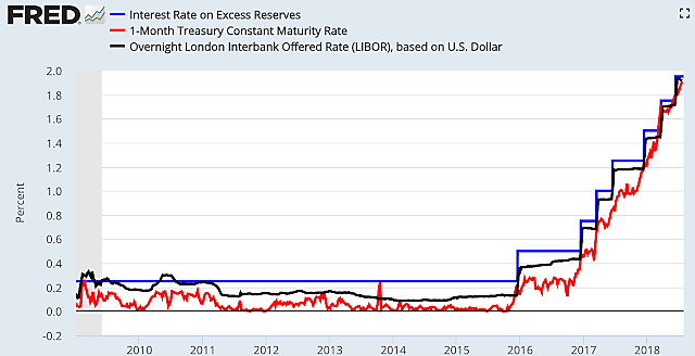
Since 2008 the Fed has used Interest of Excess Reserves (IOER) policy to control the quantity of bank reserves that are loaned out into the real economy. IOER is the interest rate the Fed pays member banks to sequester their reserves instead of lending them.
Since IOER interest is risk-free, safer than U.S. Treasuries since the Fed simply creates the interest paid out of thin air, banks are prone to sequester their reserves so long as the rate is attractive enough discounting for its zero-risk premium.
During the entire post-2008 period the Fed consistently paid a higher IOER rate than banks could earn on competing safe, short-term securities like 1-week, 1-month, or even 3-month Treasuries. This achieved its goal of loading banks up with trillions of dollars in reserves during the crisis to enhance their liquidity positions while preventing those reserves from being unleashed on the real economy and sparking runaway inflation.
https://www.cato.org/sites/cato.org/files/styles/pubs_2x/public/download-remote-images/cdn.alt-m.org/277165213523/DB_altm1.png?itok=KcDSesq-
The Fed will use the IOER rate as its primary policy tool during and after the coronavirus crisis as well. If the Fed sees inflationary pressures building, it will raise the IOER rate to impel banks to moderate lending enough to restrain the inflation rate.
Over the next several quarters the Economics Correspondent will monitor increases in monetary aggregates and compare them against changes in real GDP and velocity. While unwilling to bet his life's savings on it, he anticipates:
-Higher monetary aggregates
-An initial sharp GDP contraction followed by a slower recovery (although rapid compared to previous recoveries due simply to the size of the initial contraction)
-An even sharper contraction in velocity that persists long after GDP bottoms out.
No comments:
Post a Comment
Note: Only a member of this blog may post a comment.