Inflation and Deflation Fallacies Part 3: Why So Many Economists Get Deflation Wrong

 Click here to read the original Cautious Optimism Facebook post with comments

4/6 MIN READ - The Cautious Optimism Correspondent for Economic Affairs and Other Egghead Stuff continues discussing inflation and deflation fallacies by explaining why so many economists just don’t understand deflation.

As we demonstrated in the Correspondent’s previous installment on deflation, zero inflation or gently falling prices don’t cause or prolong recessions and depressions. And the USA has 138 years of history before 1914 to prove it, when prices gently fell throughout and the economy grew at breakneck speed into the world’s largest.

You can read that article at:

http://www.cautiouseconomics.com/2020/09/inflation-currencies06.html

But in the meantime, how then could so many mainstream economists and the media (restrain laughter) get deflation so wrong?

As monetary economist George Selgin of the CATO Institute never tires of explaining, most economists don’t understand the difference between good deflation and bad deflation.

V. CLEARING UP THE THEORETICAL MISTAKE: BAD (VERSUS GOOD) DEFLATION

So what’s bad deflation?

Bad deflation is rapidly falling prices associated with a catastrophic shock to demand, typically the result of the many banking crises that occurred throughout the 19th century and during the Great Depression.

When banks fail in large numbers their demand deposit (ie. checkbook) balances become worthless and the money supply suffers a sudden contraction. Furthermore, during a crisis even surviving banks tighten up credit and curtail lending—a measure to conserve scarce reserves. 

As debtors pay back debts but no new loans are made, the money supply further contracts, so all other things being equal prices fall.

The most famous case of bad deflation, which virtually all mainstream economists cite, is the 1930-1933 period of the Great Depression when 10,000 U.S. banks failed, the money supply shrank by one-third, and prices fell a whopping 10% per year on average for nearly four years.

In a deflation that extreme, not only were prices falling very rapidly but the bank failures themselves and associated drying up of lending harmed the economy even more. In other words, it wasn’t so much falling prices themselves that were tanking the economy, but rather a collapsing financial system. Rapid price deflation, while certainly problematic, was as much a consequence as a cause of depression.

In such a scenario debt can also becomes a problem since debt payments are fixed in nominal terms but prices and wages quickly fall so more borrowers default, placing even more strain on the credit system.

This is pretty much all most economists think of when they consider falling prices. They're taught, and believe, that deflation of any kind must necessarily produce Great Depression conditions.

VI. BAD DEFLATION MAY NOT BE QUITE THAT BAD AFTER ALL

Yet as bad as the 1930’s deflation scenario is, assumptions about the extent of its malignance have to be questioned because there is historical precedent of rapid deflation that didn’t produce a Great Depression.

After the mostly-forgotten Panic of 1839, prices also fell by even more than one-third over four years in a deflation that exceeded the Great Depression’s. 

But the macroeconomic results were quite different then. As Professor Jeffrey Rogers Hummel of San Jose State University writes:

“During the Great Depression, as unemployment peaked at 25 percent of the labor force in 1933, U.S. production of goods and services collapsed by 30 percent. During the earlier nineteenth-century contraction [1839-1843], investment fell, but amazingly the economy's total output did not. Quite the opposite; it actually rose between 6 percent and 16 percent. 

"This was nearly a full-employment deflation. Nor are economists at any loss to account for this widely disparate performance. The American economy of the 1930s was characterized by prices, especially wages, that were rigid downward, whereas in the 1840s, prices could fall fast and far enough to quickly restore market equilibrium.”

-“Martin Van Buren: The American Gladstone” by Jeffrey Rogers Hummel

Even mainstream MIT former Economics Department Chair Peter Temin, himself a fairly left-leaning mainstream quasi-Keynesian cites the 1839-1843 experience:

“As some detailed estimates by economic historian Peter Temin show, the contraction in the money supply was even greater in 1839-43 than in 1929-33. The fall in the price level was substantially greater: -31 percent in 1929-33 and -42 percent in 1839-43.

"But consumption in real terms, which decreased by 19 percent in 1929 to 1933 increased 21 percent from 1839 to 1843. More dramatically still the real gross domestic product, which decreased by no less than 30 percent from 1929 to 1933, increased by 16 percent from 1839 to 1843.”

-“The Rise and Decline of Nations” by Mancur Olson

To add color to Professor Hummel’s contrast between the price and wage policies of the 1839-1843 and 1929-1933 periods, the Correspondent would like to add that during the Hoover years of the Great Depression the top federal tax rate was raised from 25% to 63%, taxes on the middle classes raised by over 100%, an international trade war was launched by the Smoot-Hawley Tariff, and federal government spending more than doubled in real terms.

So while the Economics Correspondent doesn’t want to test the theory of 10% annual deflation anytime soon, the stark contrast between the 1839-1843 and 1929-1933 periods suggests free market economies are more resilient to rapidly falling prices than mainstream economists believe. 

An over 40% fall in prices during the 19th century failed to produce a Great Depression because market prices and wages were freely floating and allowed to adjust rapidly.  And 19th century America was free from the crushing government tax and spending hikes, inflexible labor regulations, and global trade wars of the 1930's.

VII. CLEARING UP THE THEORETICAL MISTAKE: GOOD DEFLATION

However there is a “good” kind of deflation too, and it dominated the 19th century with the exception of several banking panics that occurred on average every dozen years.

Good deflation occurs when the economic output is growing faster than the money supply. 

During the 19th century the United States was on a bimetallic (gold and silver) standard until 1879 when it joined the industrialized world on the monometallic classical gold standard. But in both cases, the money supply was closely linked to precious metal reserves and the pace of new mining discoveries thus limiting the rate of monetary expansion.

If, for example, the economy produced 5% more goods and services one year but the money supply, constrained by the gold standard, grew by only 4%, then assuming constant velocity the price level fell roughly 1% (104 units of new money divided by 105 new units of product = 99.05% the previous price level).

Quite the opposite from the bad deflation scenario, good inflation is associated with strong economic growth. Clearly the faster the economy grows the further prices will fall provided money growth remains restrained, or in the Equation of Exchange mv = py, rising output ( y ) results in a lower price level ( p ), all other variables being equal.

In real world practice this produced benign, gentle deflation during the Gilded Age. Annual prices fell a little slower than 1% on average from 1865 to 1914, and far from a half-century Great Depression America experienced the fastest half-century of economic growth in its history.

Unfortunately most economists are taught in school that depression is simply associated with deflation, particularly the Great Depression. They also look at the recessions and depressions of the 19th century and notice an accompanying fall in prices—a trend present throughout the entire century, not just during slumps—and conclude deflation must have caused those downturns.

Well correlation is not causation, as deflation was the norm during both economic booms and economic busts during the pre-Fed era.

And one mustn’t underestimate the impact of living in an academic and media echo chamber, where large numbers of intellectuals and reporters simply recycle the myth among themselves. 

The myth, repeated enough times, becomes the truth, although the Economics Correspondent doesn’t let academia in particular off the hook. It’s their job to thoroughly research the theory and history before opining. Too many don’t.

====OK, stop reading here unless you are an econ nerd seeking a more detailed (wonkish) analysis.====

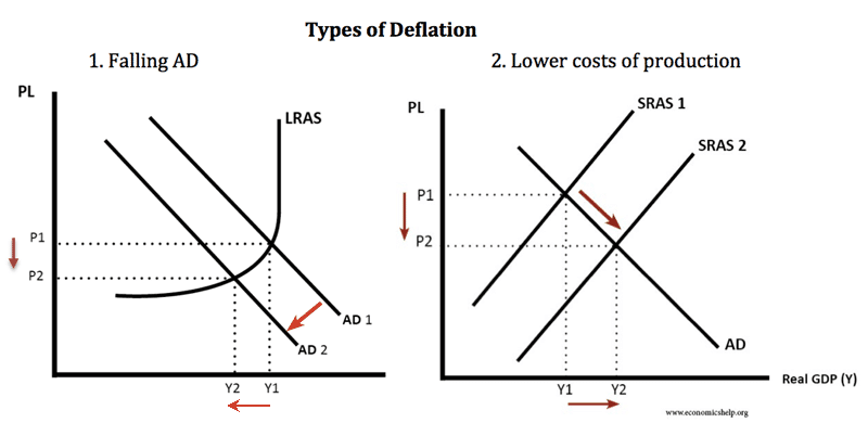
ps. See attached visual model of good vs bad deflation.

https://www.economicshelp.org/wp-content/uploads/2017/11/types-of-deflation-1.png

Model 1 (“Falling AD”) is a graph of bad deflation resulting from a sudden demand shock, usually the result of a banking crisis and contracting money supply. The quantity (x-axis) of demand represented by curve AD1 shifts left to lesser demand curve AD2. Thus the intersection with long-run aggregate supply curve LRAS moves down the price or y-axis from P1 to P2 resulting in lower prices.

Model 2 (“Lower costs of production”) is a graph of good deflation resulting from capital investment and higher productivity which raises output of goods and services per unit of labor. The quantity (x-axis) of aggregate supply represented by curve SRAS1 shifts right to greater supply curve SRAS2. Thus the intersection with aggregate demand curve AD moves down the price or y-axis from P1 to P2 resulting in a lower prices.

There is absolutely nothing wrong with Model 2 as it was the real-world norm during the spectacular growth periods of the Industrial Revolution and American Gilded Age. In fact good deflation would be the norm today were it not for central banks producing new money at a rate faster than the growth of goods and services in a deliberate policy of eternal price inflation.

In the “bad deflation” environment, government intervention has historically made things much worse. If the government forces prices back to P1 (price and wage floors such as those during the Great Depression) a gap or “surplus” in quantity appears between new demand curve AD2 and supply curve LRAS. That gap—follow dotted-line P1 between AD1 and AD2—in quantity applies to both goods and services and particularly labor. 

Hence as aggregate demand fell during the Great Depression and the government forced wages up to old price level P1, the supply of labor at LRAS/P1 exceeded the demand for labor at AD2/P2, and the surplus was manifested as double-digit unemployment for a decade that peaked above 25% in 1933.